Determination of specific losses due to magnetization reversal of iron. Magnetic losses
GOST 12119.4-98
Group B39
INTERSTATE STANDARD
Electrical steel
METHODS FOR DETERMINING MAGNETIC AND ELECTRIC PROPERTIES
Method for measuring specific magnetic loss and effective value
magnetic field strength
electrical steel.
Methods of test for magnetic and electrical properties.
Method for measurement of specific magnetic losses
and actual value of magnetic field intensity
MKS 77.040.20
OKSTU 0909
Introduction date 1999-07-01
Foreword
1 DEVELOPED by the Russian Federation, Interstate Technical Committee for Standardization MTK 120 "Metal products from ferrous metals and alloys"
INTRODUCED by Gosstandart of Russia
2 ADOPTED by the Interstate Council for Standardization, Metrology and Certification (Minutes No. 13 of May 28, 1998)
Voted to accept:
State name | Name of the national standardization body |
The Republic of Azerbaijan | Azgosstandart |
Republic of Armenia | Armstate standard |
Republic of Belarus | State Standard of Belarus |
Kyrgyz Republic | Kyrgyzstandart |
the Russian Federation | Gosstandart of Russia |
The Republic of Tajikistan | Tajik State Standard |
Turkmenistan | Main State Inspectorate of Turkmenistan |
The Republic of Uzbekistan | Uzgosstandart |
Ukraine | State Standard of Ukraine |
3 By Decree of the State Committee of the Russian Federation for Standardization and Metrology dated December 8, 1998 N 437, the interstate standard GOST 12119.4-98 was put into effect directly as the state standard of the Russian Federation from July 1, 1999.
4 INSTEAD OF GOST 12119-80 in part of section 4
5 REVISION
1 area of use
1 area of use
This standard establishes a method for determining specific magnetic losses from 0.3 to 50.0 W/kg and the effective value of the magnetic field strength from 100 to 2500 A/m at remagnetization frequencies of 50-400 Hz using the wattmeter and ammeter method.
It is allowed to determine the values of magnetic quantities at remagnetization frequencies up to 10 kHz on ring samples and on samples from strips.
2 Normative references
This standard uses references to the following standards:
GOST 8.377-80 State system for ensuring the uniformity of measurements. The materials are soft magnetic. Methods for performing measurements when determining static magnetic characteristics
GOST 8476-93 Direct-acting analog indicating electrical measuring instruments and auxiliary parts to them. Part 3: Particular requirements for wattmeters and varmeters
GOST 8711-93 Direct-acting analog indicating electrical measuring instruments and auxiliary parts to them. Part 2: Particular requirements for ammeters and voltmeters
GOST 12119.0-98 Electrical steel. Methods for determining magnetic and electrical properties. General requirements
GOST 13109-97 Electrical energy. Compatibility of technical means is electromagnetic. Standards for the quality of electrical energy in general-purpose power supply systems
GOST 21427.1-83 Electrical cold-rolled anisotropic sheet steel. Specifications
GOST 21427.2-83 Electrical cold-rolled isotropic thin sheet steel. Specifications
3 General requirements
General requirements for test methods - according to GOST 12119.0.
The terms used in this standard are in accordance with GOST 12119.0.
4 Preparation of test specimens
4.1 Test specimens shall be insulated.
4.2 Ring-shaped samples are assembled from stamped rings with a thickness of 0.1 to 1.0 mm or wound from a tape with a thickness of not more than 0.35 mm and placed in cassettes of insulating material with a thickness of not more than 3 mm or non-ferromagnetic metal with a thickness of not more than 0.3 mm. The metal cassette must have a gap.
The ratio of the outer diameter of the sample to the inner should be no more than 1.3; the cross-sectional area of the sample is not less than 0.1 cm.
4.3 Samples for the Epstein apparatus are made from strips with a thickness of 0.1 to 1.0 mm, a length of 280 to 500 mm, a width of (30.0 ± 0.2) mm. The strips of the sample should not differ from each other in length by more than ± 0.2%. The cross-sectional area of the sample must be between 0.5 and 1.5 cm. The number of stripes in the sample must be a multiple of four, with a minimum of twelve stripes.
Samples of anisotropic steel are cut along the rolling direction. The angle between the directions of rolling and cutting of strips must not exceed 1° .
For samples of isotropic steel, half of the strips are cut along the rolling direction, the other - across. The angle between the rolling and cutting directions must not exceed 5°. The strips are grouped into four packages: two - from strips cut along the rolling direction, two - across. Packages with equally cut strips are placed in parallel coils of the apparatus.
It is allowed to cut strips at the same angle to the direction of rolling. The direction of rolling for all strips laid in one coil must be the same.
4.4 Sheet samples are made from 400 to 750 mm long. The length of the sheet must be at least the outer length of the yoke: the width of the sheet must be at least 60% of the width of the solenoid window. The tolerance in length should not exceed ±0.5%, in width - ±2 mm.
The surface and shape of the sheets must comply with GOST 21427.1 and GOST 21427.2.
5 Applied equipment
5.1 Installation. The installation diagram is shown in Figure 1.
Figure 1 - Scheme for measurements by the wattmeter method
5.1.1 Voltmeters PV1- to measure the average rectified voltage value and then determine the amplitude of the magnetic induction and PV2- to measure the effective voltage value and the subsequent determination of the shape factor of its curve, they must have a measurement limit from 30 mV to 100 V, a maximum input current of not more than 5 mA, an accuracy class of at least 0.5 according to GOST 8711.
It is allowed to use a voltage divider to a voltmeter PV1 to obtain readings numerically equal to the amplitudes of the magnetic induction.
5.1.2 Wattmeter PW for measuring active power and subsequent determination of specific magnetic losses, it must have a measurement limit of 0.75 to 30 W, a rated power factor of not more than 0.1 at a frequency of 50 Hz and 0.2 at a higher frequency; accuracy class not less than 0.5 at a frequency of magnetization reversal from 50 to 400 Hz or not less than 2.5 - at a frequency of more than 400 Hz according to GOST 8476.
It is allowed to use a voltage divider to the wattmeter to obtain readings numerically equal to the values of specific magnetic losses. The output of the voltage divider must be connected to the parallel circuit of the wattmeter, the input - to the winding II of the sample T2.
5.1.3 Ammeter RA to measure the effective value of the magnetizing current and the subsequent determination of the effective value of the magnetic field strength, it must have a measurement limit from 0.1 to 5.0 A, an accuracy class of at least 0.5 according to GOST 8711. It is allowed to increase the smallest measurement limit up to 1.0 A when controlling the load of the current circuit of the wattmeter. The maximum power consumed by the ammeter when measuring with samples from sheets with a width of more than 250 mm should be no more than 1.0 VA; for other samples - no more than 0.2 VA.
5.1.4 Frequency counter PF for measuring frequency with an error not exceeding ±0.2%.
5.1.5 The power source for sample magnetization should have a low-frequency generator with a power amplifier or a voltage regulator with a 50 Hz frequency stabilizer. The coefficient of non-sinusoidal voltage of the loaded power source should not exceed 5% according to GOST 13109. The rated power of the source at a remagnetization frequency of 50 Hz must be at least 0.45 kVA per 1.0 kg of sample weight and at least 0.3 kVA for the values specified in Table 1.
Table 1
Remagnetization frequency, kHz | Sample weight, kg |
From 0.05 to 1.0 incl. | From 0.5 to 1.1 incl. |
St. 1.0 "10.0" | From 0.03" to 0.30" |
It is allowed to use a feedback amplifier to obtain the shape of the magnetic flux curve of the sample, close to sinusoidal. The coefficient of non-sinusoidality of the shape of the EMF curve in the winding should not exceed 3%; the power consumed by the voltage feedback circuit must not exceed 5% of the measured magnetic losses.
5.1.6 Voltmeters PV1 and PV2, wattmeter voltage circuit PW and amplifier feedback should consume no more than 25% of the measured value.
5.1.7 Coil T1 to compensate for the magnetic flux outside the sample, the number of turns of the winding I should not exceed fifty, the resistance should not exceed 0.05 ohms, the resistance of the winding II should not exceed 3 ohms. The windings are laid on a cylindrical frame made of non-magnetic insulating material with a length of 25 to 35 mm and a diameter of 40 to 60 mm. The axis of the coil must be perpendicular to the plane of the lines of force of the sample when it is fixed on the Epstein apparatus. Relative difference between the coefficients of mutual inductance of the coil T1 and the Epstein apparatus without sample should not go beyond ± 5%.
It is allowed to exclude from the circuit (see Figure 1) the coil T1 with a magnetic flux outside the sample not exceeding 0.2% of the measured value.
5.1.8 Magnetizing I and measuring windings II of the annular sample T2 must comply with the requirements of GOST 8.377.
5.1.9 Epstein apparatus, used to test specimens composed of strips, T2 shall have four coils on frames of non-magnetic insulating material with the following dimensions:
inner window width - (32.0±0.5) mm;
height - from 10 to 15 mm;
frame wall thickness - from 1.5 to 2.0 mm;
the length of the section of the coil with the winding is not less than 190 mm;
coil length - (220±1) mm.
The number of turns in the windings of the apparatus is selected in accordance with Table 2.
table 2
Remagnetization frequency, Hz | The number of turns in the winding |
|
I - magnetizing | II - measuring |
|
From 50 to 60 incl. St. 60 "400" " 400 " 2000 " | ||
Note - The windings are wound evenly along the length of the coil frames. The number of layers of each winding on the frames must be odd. |
||
5.1.10 Sheet apparatus used for testing specimens T2, must have a solenoid and two yokes. The design of the yokes must ensure the parallelism of the contacting surfaces and mechanical rigidity, which excludes the influence on the magnetic properties of the sample. The width of the poles of electrical steel yokes must be at least 25 mm, those of precision alloys - 20 mm. Magnetic losses in the yokes should not exceed 5% of the measured ones; the relative difference of the amplitudes of the magnetic flux in the yokes should not go beyond ±15%.
It is allowed to use devices with open yokes to measure the relative change in specific magnetic losses, for example, when assessing the residual voltage according to GOST 21427.1.
The solenoid must have a frame made of non-magnetic insulating material, on which the measuring winding II is first placed, then the magnetizing winding I is placed with one or more wires. Each wire is evenly laid in one layer.
The relative maximum difference in the amplitudes of the magnetic induction in the area of the sample inside the solenoid should not go beyond ±5%.
6 Preparing for measurements
6.1 Samples from strips, sheets or annular shapes are connected as shown in figure 1.
6.2 Samples from strips or sheets are placed in the apparatus. Samples from the strips are placed in the Epstein apparatus, as indicated in Figure 2.
Figure 2 - Scheme of laying strips of the sample
It is allowed to fix the position of the strips and sheets in the apparatus, creating a pressure of not more than 1 kPa perpendicular to the surface of the sample outside the magnetizing coils.
6.3 Calculate the cross-sectional area, m, of the samples:
6.3.1 The cross-sectional area, m, for annular-shaped samples of a material with a thickness of at least 0.2 mm is calculated by the formula
where -
sample weight, kg;
- outer and inner diameters of the ring, m;
- material density, kg/m.
The density of the material, kg / m, is selected according to Appendix 1 of GOST 21427.2 or calculated by the formula
where and -
mass fractions of silicon and aluminum, %.
6.3.2 The cross-sectional area, m, for annular specimens of a material with a thickness of less than 0.2 mm is calculated by the formula
where is the ratio of the density of the insulating coating to the density of the sample material,
where is the insulation density, taken equal to 1.6 10 kg / m for an inorganic coating and 1.1 10 kg / m for an organic one;
- fill factor, determined as specified in GOST 21427.1
6.3.3 Cross-sectional area S, m, samples made up of strips for the Epstein apparatus, calculated by the formula
where is the length of the strip, m.
6.3.4 The cross-sectional area of the sheet sample, m, is calculated by the formula
where is the length of the sheet, m.
6.4 The error in determining the mass of the samples should not exceed ±0.2%, the outer and inner diameters of the ring - ±0.5%, the length of the strips - ±0.2%.
6.5 Measurements at a magnetic induction amplitude value of less than 1.0 T are carried out after demagnetization of the samples in a field with a frequency of 50 Hz.
Set the voltage corresponding to the amplitude of the magnetic induction of at least 1.6 T for anisotropic steel and 1.3 T for isotropic steel, then gradually reduce it.
The demagnetization time must be at least 40 s.
When measuring magnetic induction in a field with a strength of less than 1.0 A/m, the samples are kept after demagnetization for 24 hours; when measuring induction in a field with a strength of more than 1.0 A / m, the exposure time can be reduced to 10 minutes.
It is allowed to reduce the exposure time with a relative difference between the induction values obtained after normal and reduced exposures, within ± 2% .
6.6 The upper limits of the values of the measured magnetic quantities for the samples of an annular shape and composed of strips must correspond to the amplitude of the magnetic field strength of not more than 5 10 A/m at a magnetization reversal frequency of 50 to 60 Hz and not more than 1 10 A/m - at higher frequencies; lower limits - the smallest values of the amplitudes of magnetic induction, given in table 3.
Table 3
Remagnetization frequency, kHz | The smallest value of the amplitude of magnetic induction, T, when measuring |
|
specific magnetic losses, W/kg | magnetic field strength, A/m |
|
From 0.05 to 0.06 incl. | ||
St. 0.06 "1.0" | ||
" 1,00 " 10,0 " | ||
The smallest value of the magnetic induction amplitude for sheet samples should be equal to 1.0 T.
6.7 For voltmeter PV1, calibrated in medium-rectified values, voltage, V, corresponding to a given amplitude of magnetic induction, T, and magnetization reversal frequency, Hz, is calculated by the formula
where -
cross-sectional area of the sample, m;
- the number of turns of the winding of the II sample;
- total winding resistance of sample II T2 and coils T1, Ohm;
- equivalent resistance of devices and devices connected to the winding of sample II T2, Ohm, calculated by the formula
where -
active resistances of voltmeters PV1, PV2, wattmeter voltage circuit PW and voltage feedback circuits of the power amplifier, respectively, Ohm.
The value in formula (6) is neglected if its value does not exceed 0.002.
6.8 For voltmeter PV1, calibrated in the operating values of the voltage of a sinusoidal form, the value of the value U, V, calculated according to the formula
6.9 Without coil T1 calculate the correction , V, due to the magnetic flux outside the sample, according to the formula
where is the number of turns of the sample windings T2;
- magnetic constant, H/m;
- cross-sectional area of the measuring winding of the sample, m;
is the cross-sectional area of the specimen, determined as specified in 6.3, in m;
- the average length of the magnetic field line, m.
For annular samples, the average length of the magnetic field line, m, is calculated by the formula
In standard tests for a sample of strips, the average length, m, is taken equal to 0.94 m. If it is necessary to improve the accuracy of determining magnetic quantities, it is allowed to choose values from table 4.
Table 4
Magnetic field strength, A/m | Average length of magnetic field line, m |
|
for isotropic steel | for anisotropic steel |
|
0 to 10 inclusive St. 10 "70" | ||
For a sheet sample, the average length of the magnetic field line, m, is determined by the results of the metrological certification of the installation;
- current amplitude, A; calculated depending on the amplitude of the voltage drop, V, on a resistor with a resistance, Ohm, included in the magnetizing circuit, according to the formula
or according to the average rectified value of EMF, V, induced in the winding II of the coil T1 when the winding I is included in the magnetizing circuit, according to the formula
where -
mutual inductance of the coil, H; no more than 1 10 Gn;
- remagnetization frequency, Hz.
6.10 When determining the specific magnetic losses in the Epstein apparatus, one should take into account the inhomogeneity of the magnetization of the corner parts of the magnetic circuit by introducing the effective mass of the sample, kg, which for samples from strips is calculated by the formula
where -
sample weight, kg;
- strip length, m.
For annular samples, the effective mass is assumed to be equal to the mass of the sample.
The effective mass of the sheet sample is determined by the results of the metrological certification of the installation.
7 Measurement procedure
7.1 Determination of specific magnetic losses is based on the measurement of active power consumed by the magnetization reversal of the sample and consumed by devices PV1, PV2, PW and amplifier feedback circuit. When testing a sheet sample, losses in yokes are taken into account. Active power is determined indirectly by the voltage on the winding of the II sample T2.
7.1.1 At the installation (see Figure 1), the keys are closed S2, S3, S4 and open the key S1.
7.1.2 Set the voltage, or (), V, using a voltmeter PV1; remagnetization frequency, Hz; check with an ammeter RA, what is the wattmeter PW not overloaded; close the key S1 and open the key S2.
7.1.3 If necessary, adjust the voltmeter reading with the power source PV1 to set the set voltage value and measure the effective voltage value, V, with a voltmeter PV2 and power, W, wattmeter P.W.
7.1.4 Set the voltage corresponding to the larger value of the amplitude of the magnetic induction, and repeat the operations specified in 7.1.2, 7.1.3.
7.2 Determination of the effective value of the magnetic field strength is based on the measurement of the magnetizing current.
7.2.1 At the installation (see Figure 1), the keys are closed S2, S4 and unlock the keys S1, S3.
7.2.2 Set the voltage or u, V, remagnetization frequency, Hz, and determined by an ammeter RA values of the magnetizing current, A.
7.2.3 Set a higher voltage value and repeat the operations indicated in 7.2.1 and 7.2.2.
8 Rules for processing measurement results
8.1 The shape factor of the voltage curve on the winding II of the sample is calculated by the formula
where -
effective voltage value, V;
-
voltage calculated by formula (6), V.
8.2 Specific magnetic loss, W / kg, of a sample from strips or an annular shape is calculated by the formula
where is the effective mass of the sample, kg;
- average value of power, W;
- effective voltage value, V;
- the number of turns of the sample windings T2;
- see 6.7.
The values and are neglected if the ratio does not exceed 0.2% of and the ratio does not exceed 0.002.
The error in determining the resistance should not go beyond ± 1%.
It is allowed to substitute a value equal to 1.11 instead of voltage at =
1,
In variable fields, the area of the hysteresis loop increases due to hysteresis losses R g, eddy current losses R in and additional losses R d. Such a loop is called dynamic, and the total losses are full or total. Hysteresis loss per unit volume of material (specific loss) (W/m3)
|
(8.10) |
The same losses can be attributed to a unit of mass (W / kg)
|
(8.11) |
where g - material density, kg / m 3
To reduce hysteresis losses, magnetic materials with as little coercivity as possible are used. For this, internal stresses in the material are removed by annealing, the number of dislocations and other defects is reduced, and the grains are enlarged.
Eddy current loss for sheet specimen
|
|
(8.12) |

where
Bmax - amplitude of magnetic induction, T ;
f- AC frequency, Hz;
d- sheet thickness, m;
g- density, kg / m 3 ;
r- electrical resistivity, Ohm. m.
Additional losses or losses due to magnetic viscosity (magnetic aftereffect) are usually found as the difference between the total losses and the sum of the losses due to hysteresis and eddy currents
where J no– magnetization at t ® ¥ ; t - relaxation time. Figure 8.14 shows the dependence of the magnetic field strength and magnetization on the duration of the magnetic field. In hard magnetic materials, time t magnetic relaxation can reach several minutes. This phenomenon is called superviscosity.

Fig.8.14. Magnetization dependence J and strength H of the magnetic material on the time of action of the magnetic field t
These losses are primarily due to the inertia of the domain magnetization reversal processes (the expenditure of thermal energy for moving the boundaries of weakly pinned domains with a change in the field).
When magnetization is reversed in an alternating field, a phase lag occurs V from H magnetic field. This happens as a result of the action of eddy currents that prevent, in accordance with Lenz's law, a change in magnetic induction, as well as due to hysteresis phenomena and magnetic aftereffect.
δ m - lagging angle - the angle of magnetic losses.
tg δm is a characteristic of the dynamic properties of magnetic materials.
The tangent of the magnetic loss angle is used in alternating fields. It can be expressed in terms of the equivalent circuit parameters shown in Figure 8.15. An inductive coil with a core of magnetic material is represented as a series circuit of inductance L and active resistancer.

Rice. 8.15. Equivalent circuit (a) and vector diagram (b) of an inductive coil with a magnetic core
Neglecting its own capacitance and the resistance of the coil winding, we obtain
|
tg d m = r/(w L) |
(8.15) |
Active power R a:
|
R a=J2. w L. tg d m . |
(8.16) |
The reciprocal of tg d m called the quality factor
1Timofeev I.A.
On iron-silicon alloys, the resistivity was studied as a function of the dislocation density and domain concentration. The use of specific losses at magnetization induction of 1.0 and 1.5 T for iron-silicon alloys Fe-4% Si and Fe-6.5% Si was studied. The necessary practical information, comparative data and test results are given, which can be used to select the necessary manufacturing technology. The developed innovative technology of magnetic circuits can be applied in a technical solution in the manufacture of magnetic systems of various electrical products.
In electrical units such as generators, motors, generator-motor systems, transformers, magnetic amplifiers, electromagnets of contactors and magnetic starters, the main task is the distribution, amplification and conversion of electromagnetic energy. This requires the use of materials with low losses and high saturation induction in magnetic systems for them. These requirements are best met by iron-silicon alloys.
Doping with silicon, which forms a substitutional solid solution with iron, causes an increase in electrical resistivity. The effect of silicon on electrical resistivity is determined by the following approximate empirical formula:
Iron-silicon alloys with low values of electrical resistivity are not widely used even in low-frequency technology due to increased eddy currents. The magnitude and direction of eddy currents, in addition to the size of the magnetic core, is affected by its electrical resistivity, frequency of the electric current and magnetic permeability. Accordingly, eddy currents caused by magnetization reversal of magnetic materials affect specific electrical losses.
Refinement of the calculation formula
Modern formulas for calculating specific losses give certain errors. Let's look at this with examples.
An attempt to calculate the specific losses due to eddy currents in a ferromagnet was made in 1926 by B.A. Vvedensky. He proposed the following formula:
![]() , (2)
, (2)
where d is the plate thickness;
In o - magnetic induction, In o =m×H o;
ω - cyclic frequency;
q - magnetic conductivity.
However, formula (2) very approximately determines the specific eddy current losses. Vvedensky's mistakes were that the value of the magnetic conductivity q had to be entered in the numerator, and not in the denominator. In addition, it was necessary to enter the value of the cyclic frequency into the numerator not to the first degree, but to the second, i.e. w 2 , and in the denominator it was necessary to take into account the value of the density of the material.
Interest in the determination of specific losses in magnetic materials arose in connection with the possibility of their wide application in the creation of hot-rolled electrical steel for electrical machines. After Goss discovered high magnetic properties in 1935 in cold-rolled electrical steel along the rolling direction, interest in the study of specific losses increased. In subsequent years, research to improve the electrical characteristics of steel is intensified.
The first approximate semiphenomenological equation for calculating total losses in a conducting ferromagnet was given in 1937 by Elwood and Legg:
R full = ![]() , (3)
, (3)
where B is a constant value for a given alloy;
μ - magnetic permeability;
C is a value independent of B o and w.
Experimental verification showed that the errors of Elwood and Legg consisted in the fact that, in addition to those errors that were made by Vvedensky, it was necessary to introduce the values of the density of the material and the coercive force into the approximate semiphenomenological equation (3). Entered parameters B 0 3 and μ 3 into equation (3) additionally distort the calculation results.
The above formula (3) does not take into account the dislocation theory of the magnetic properties of materials. A more accurate dependence of the definition of energy losses on physical quantities during the magnetization reversal of a ferromagnet was given by Mishin:
![]() , (4)
, (4)
where is the magnetostrictive constant;
l is the average thickness of the dislocation segment;
δ is the thickness of the domain structure;
c - Burgers vector;
N is the density of dislocations;
S is the area of shifting domain boundaries;
n is the number of domains in a unit volume of a ferromagnet.
This dependence takes into account the absorption of energy by domain walls with dislocation segments bending under the action of an elastic field, but does not take into account the hysteresis component of losses and does not take into account the electrical resistivity of the material. However, this dependence makes it possible to determine the energy losses from physical quantities and does not allow one to practically determine the specific losses on industrial magnetic materials depending on technical quantities.
A practical formula for engineering calculations of specific electrical losses due to eddy currents was proposed by Krug. He, summing up the set of closed electrical circuits, took into account the losses in all circuits and gave the following expression:
R in = ![]() , (5)
, (5)
where In m - the amplitude of the magnetic induction, T;
f- frequency of alternating current, Hz;
d - plate thickness, mm;
k f - shape factor of the magnetic induction curve;
γ is the density of the plate material, kg/m 3 ;
ρ - specific electrical resistance of the plate material, Ohm×m.
Applying formula (5), the results of practical calculations become underestimated on average by four orders of magnitude, i.e. 10 4 times.
However, in order for formula (5) to be fully represented in the SI system and correspond approximately to real indicators for eddy current losses, it is necessary to substitute the thickness of the plates in meters into the formula and cancel the coefficient 10 -10, i.e.:
R in = ![]() . (6)
. (6)
It is known from Druzhinin's work that the hysteresis losses are proportional to the area of the statistical hysteresis cycle, the magnetization reversal frequency and are inversely proportional to the density of the plate material, and are determined from the following expression:
where S is the area of the static hysteresis cycle, T × a/m.
By converting the hysteresis loop into a rectangle, the area of the static hysteresis loop can be approximated by the following simple formula:
S= 4V m × H s, (8)
where H c is the coercive force.
Therefore, the specific hysteresis losses, taking into account formula (8), can be determined by the following formula:
Having determined the loss components by formulas (6) and (9), we can find the total specific losses for magnetization reversal of magnetically soft materials:
P \u003d P in + P g \u003d  , (10)
where H c - the value of the coercive force is given without taking into account the density of dislocations and the concentration of domains.
Based on the modern dislocation theory of magnetic properties of materials, the coercive force is influenced by the interaction of the domain and dislocation structures. For this case, the coercive force can be represented as:
H c \u003d 1.5  , (11)
Here K is the magnetic anisotropy constant; δ is the thickness of the domain wall; μ 0 - magnetic constant, μ 0 \u003d 4p × 1 0 -7 Gn / m; I S - spontaneous magnetization; D is the crystallite diameter; N is the current density of dislocations; N about - the maximum density of dislocations; c 1 - constant for the dislocation density ratio; n is the current concentration of domains; n about - the maximum concentration of domains; c 2 is a constant for the domain concentration ratio.
Therefore, finally, the total specific losses, taking into account formula (11), can be represented by the following formula.
P=  . (12)
The electrical resistivity of a magnetic material is a structurally sensitive quantity. We write the equation for the dependence of the electrical resistivity on the dislocation density and domain concentration in the following form, taking into account equation (1):
 . (13)
where c is the coefficient, c=0.1...0.9;
q is a constant for the dislocation density ratio;
ε is a constant for the domain concentration ratio.
The electrical resistivity of a magnetic material is affected by the interaction of the domain and dislocation structures.
Objects and methods of research
Tests to determine the electrical resistivity were subjected to cylindrical samples of Fe-4% Si and Fe-6.5% Si alloys with a length of 65 × 10 -3 m, a diameter of 6 + 0.2 ×10 -3 m, the manufacturing technology of which was carried out according to the method. Sampling was performed according to GOST 20559.
Measurement of electrical resistivity was carried out according to the method described in GOST 25947. As a device, a direct current potentiometer of the R-4833 type with a measurement limit of 1×10 -2 to 1×10 4 Ohm was used. The accuracy class of the instrument was 0.05.
The measurement method consists in passing a constant electric current through the alloy and determining the voltage drop over a known section of its length. The specific electrical resistance was calculated by the formula:
where U is the voltage drop between the contacts, V;
S is the cross-sectional area of the sample, mm 2;
I is the strength of the current flowing through the sample.
L - distance between contacts.
The study and modification of structural defects was carried out by irradiating samples with gamma rays of radioactive elements having a wavelength in the range of 1×10 -1 ¸3×10 -3 nm. For this purpose, a stationary X-ray apparatus of the TUR-D-1500 type with a radiation energy of 150 keV was used.
Metallographic studies, as well as registration of the dislocation structure, were carried out on MIM-8 and Neofot-32 metallographic microscopes, and a BS-613 electron microscope with an accelerating voltage of 100 kV was used to control dislocations.
The objects for studying the specific electrical losses were samples 0.28 m long, 0.03 m wide, 0.5×10 -3 m thick. The characteristics were taken at a given induction amplitude of 1.0 and 1.5 T. The error was 3%.
The determination of specific electrical losses was carried out in accordance with GOST 12119 on a small Epstein apparatus (samples weighing 1 kg) at a low industrial frequency of 50 Hz. The device was used in a set with the following measuring instruments: F-585 electronic wattmeter, GZ-34 sound generator, F-564 electronic millivoltmeter and VZ-38 tube millivoltmeter.
Experimental results
For the physics of magnetic materials, it is of theoretical interest to study the effect of dislocation density on electrical resistivity.
Experimental tests have shown that the electrical resistivity of the samples with a high measure of accuracy is structurally sensitive to the appearance of defects in them. With an increase in the dislocation density, the electrical resistivity increases adequately. With an increase in the dislocation density by one order of magnitude from 6×10 11 to 6×10 12 m -2, the electrical resistivity increases for a sample of Fe-4% Si alloy from 0.9 to 2.2 Ohm×m, i.e. 2.4 times, and for a sample of Fe-6.5% Si alloy from 1.2 to 2.6 Ohm×m, i.e. 2.3 times.
Of practical interest is the determination of the dependence of specific losses on the density of dislocations and the quantitative content of silicon at various magnetization inductions. The influence of the dislocation structure on the specific losses was studied in alternating magnetic fields with a power frequency of 50 Hz. The figure shows in logarithmic coordinates the results of measurements of specific losses depending on the dislocation density. With an increase in the dislocation density by one order of magnitude from 2×10 11 to 2×10 12 m -2, the specific losses increase within the following limits: for a sample of Fe-4% Si alloy at a magnetic induction of 1.5 T from 3.3 to 9 0 W/kg, i.e. by 2.7 times, for a sample of Fe-6.5% Si alloy at a magnetic induction of 1.5 T from 1.8 to 5.8 W / kg, i.e. 3.2 times; for a sample of Fe-4% Si alloy at a magnetic induction of 1.0 T from 1.2 to 3.6 W/kg, i.e. 3.0 times, for a sample of Fe-6.5% Si alloy at a magnetic induction of 1.0 T from 0.7 to 2.4 W/kg, i.e. 3.4 times.
The study of the influence of the domain concentration on the electrical resistivity is of no lesser practical interest. With an increase in the concentration of domains from 6×10 4 to 6×10 5 m -2, the electrical resistivity decreases for a sample of Fe-4% Si alloy from 2.3×10 -6 to 0.37×10 -6 Ohm×m, those. 6.1 times, and for a sample of Fe-6.5% Si alloy from 3.45×10 -6 to 0.65×10 -6 Ohm×m, i.e. 5.3 times.

Rice. one. Dependence of the specific electrical losses of iron-silicon alloys on the dislocation density at various magnetization inductions
1 - Fe-4.0% Si (1.5 T); 2 - Fe-6.5% Si (1.5 T);
3 - Fe-4.0% Si (1.0 T); 4 - Fe-6.5% Si (1.0 T);
Discussion of the results of the experiment
The change in the concentration of defects in the material can be indirectly judged by the change in electrical resistivity.
The physical essence of the phenomenon under consideration is as follows. Under the action of an electromagnetic field, relaxations of dislocations occur, which differ sharply in form from harmonic sinusoidal oscillations. The intense movement of free electrons in the metal leads to the dissipation of energy from elastic collisions with dislocations and to the excitation of the latter. The latter inhibit the passage of electric current through the metal, thereby increasing the electrical resistivity. Therefore, the occurrence of any type of dislocations in the alloy leads to an increase in electrical resistivity, and their decrease reduces the electrical resistivity. Thus, with an increase in the dislocation density by one order of magnitude, the electrical resistivity increases by a factor of 2.4 for a Fe-4% Si alloy sample, and by a factor of 2.3 for a Fe-6.5% Si sample.
An increase in specific losses occurs due to an increase in the density of dislocations. However, with an increase in the dislocation density, which leads to deterioration of the structure, the processes of displacement of the domain walls, which occur at lower magnetization inductions, become more difficult. Such an increase in the dislocation density affects the processes of domain wall rotation occurring at high magnetization inductions with a smaller multiplicity. Therefore, when the structure of the alloy deteriorates due to the increased density of dislocations, the increase in losses P 10/50 occurs with a greater multiplicity than for losses P 1.5/50.
Let us consider the influence of the domain concentration on specific losses. The fragmentary data presented in are contradictory. According to the data, there were only two domains in the square section rod. The eddy current losses were several times higher than those calculated without the participation of the domain structure of the sample. Accordingly, there were four domains in the sheet thickness. The energy losses from eddy currents were 1.5 times greater than those calculated using the well-known formula (5).
Systematic studies have shown that with an increase in the concentration of domains by one order of magnitude, the electrical resistivity decreases for a sample of Fe-4% Si alloy by 6.1 times, and for a Fe-6.5% Si sample by 5.3 times, which in total leads at a magnetization induction of 1.0 T to an increase in specific electrical losses for a sample of Fe-4% Si alloy by 3.0 times, and for a sample of Fe-6.5% Si alloy by 3.4 times, and with induction magnetization of 1.5 T to an increase in specific losses for a sample of Fe-4% Si alloy by 2.7 times, and for a sample of Fe-6.5% Si alloy by 3.2 times.
conclusions
1. A calculation formula for specific losses for magnetic materials is derived depending on the dislocation density and domain concentration.
2. It has been established that with an increase in the dislocation density by one order of magnitude, the electrical resistivity increases by 2.4 times for a sample of Fe-4% Si alloy, by 2.3 times for a sample of Fe-6.5% Si, and with an increase in the concentration of domains by one order of magnitude, the electrical resistivity decreases for a sample of Fe-4% Si alloy by 6.1 times, for a Fe-6.5% Si sample by 5.3 times, which together leads to a magnetization induction of 1.0 T to an increase in specific losses for a sample of Fe-4% Si alloy by 3.0 times, for a sample of Fe-6.5% Si alloy by 3.4 times, and with a magnetization induction of 1.5 T, to an increase in specific losses for the sample from Fe-4% Si alloy by 2.7 times, for a sample from Fe-6.5% Si alloy by 3.2 times.
BIBLIOGRAPHY:
- 1. Druzhinin V.V. Magnetic properties of electrical steel. M.: Energy, 1974. - 239 p.
- 2. Vvedensky B.A., ZhRFKhO, part of nat. 58,241 (1926).
- 3. Coss N.P. New development in electrical strip steels characterized by fine grain structure approaching the properties of a single crystal. - TASM, 1935, VI, v. 23, no. 2, p. 511-544
- 4. Elwood W.B., Legg V.E., J. Appl. Phys. 8, 351 (1937).
- 5. Mishin D.D. magnetic materials. M.: Higher school, 1991. - 384 p.
- 6. Krug K.A. Fundamentals of electrical engineering. - M.-L.: ONTI, 1936.
- 7. Timofeev I.A. Modern science-intensive technologies. - 2005. - No. 11. - S. 84-86.
- 8. Mishin D.D., Timofeev I.A. Technology of electrical production. - 1978. - No. 1 (104). - S. 1-3.
- 9. Williams H., Shockly W., Kittel C. Studies of the propagation velocity of a ferromagnetic domain boundary. - Phys. Rev., 1950, v. 80, no. 6.
- 10. Polivanov K.M. Theoretical foundations of electrical engineering. 4. III. Moscow: Energy, 1969.
- 11. Timofeev I.A., Kustov E.F. Izvestiya vuzov. Physics. - 2006. - No. 3. - S. 26. -32.
Bibliographic link
Timofeev I.A. SPECIFIC LOSSES IN A FERROMAGNET // Modern problems of science and education. - 2007. - No. 6-1 .;URL: http://science-education.ru/ru/article/view?id=753 (date of access: 01.02.2020). We bring to your attention the journals published by the publishing house "Academy of Natural History"